Description
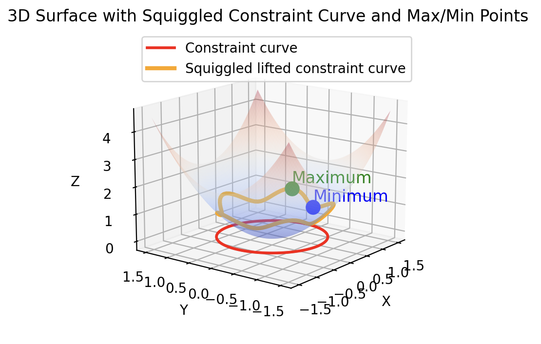
This Python script uses matplotlib to visualize a 3D surface (a paraboloid) with a squiggled constraint curve. The curve is lifted onto the surface, with two points highlighted: one at the maximum and one at the minimum of the curve. Below is an explanation of the main steps:
Image
Code
import micropip
await micropip.install("numpy")
await micropip.install("matplotlib")

import numpy as np
import matplotlib.pyplot as plt
from mpl_toolkits.mplot3d import Axes3D

# Define the surface z = f(x, y) (a paraboloid)
def f(x, y):
    return x**2 + y**2

# Set up grid for plotting
x = np.linspace(-1.5, 1.5, 400)
y = np.linspace(-1.5, 1.5, 400)
X, Y = np.meshgrid(x, y)
Z = f(X, Y)

# Create figure and 3D axis
fig = plt.figure(figsize=(6, 4))
ax = fig.add_subplot(111, projection='3d')

# Plot the surface (paraboloid)
ax.plot_surface(X, Y, Z, rstride=5, cstride=5, alpha=0.3, cmap='coolwarm')

# Plot the constraint curve at z = 0 (a circle)
theta = np.linspace(0, 2 * np.pi, 100)
r = 1  # Radius of the constraint (constant for regular curve)
x_constraint = r * np.cos(theta)
y_constraint = r * np.sin(theta)
z_constraint = np.zeros_like(x_constraint)

ax.plot(x_constraint, y_constraint, z_constraint, color='red', lw=2, label='Constraint curve')

# Modify the constraint curve to introduce "squiggle" (move radially in/out)
def squiggled_constraint(theta, base_r=1, amplitude=0.1, frequency=5):
    # Adjust radius based on sinusoidal squiggle
    r_squiggled = base_r + amplitude * np.sin(frequency * theta)
    x_squiggled = r_squiggled * np.cos(theta)
    y_squiggled = r_squiggled * np.sin(theta)
    return x_squiggled, y_squiggled

# Get the squiggled constraint curve points
x_squiggled, y_squiggled = squiggled_constraint(theta)

# Compute the corresponding z values for the squiggled curve from the surface
z_squiggled = f(x_squiggled, y_squiggled)

# Plot the squiggled lifted constraint curve
ax.plot(x_squiggled, y_squiggled, z_squiggled, color='orange', lw=3, label='Squiggled lifted constraint curve')

# Find the indices for max and min points on the squiggled curve
max_idx = np.argmax(z_squiggled)  # Index of the maximum z value
min_idx = np.argmin(z_squiggled)  # Index of the minimum z value

# Plot and label the max point
ax.scatter(x_squiggled[max_idx], y_squiggled[max_idx], z_squiggled[max_idx], color='green', s=100)
ax.text(x_squiggled[max_idx], y_squiggled[max_idx], z_squiggled[max_idx] + 0.2, 'Maximum', color='green', fontsize=12)

# Plot and label the min point
ax.scatter(x_squiggled[min_idx], y_squiggled[min_idx], z_squiggled[min_idx], color='blue', s=100)
ax.text(x_squiggled[min_idx], y_squiggled[min_idx], z_squiggled[min_idx] + 0.2, 'Minimum', color='blue', fontsize=12)

# Add labels and title
ax.set_xlabel('X')
ax.set_ylabel('Y')
ax.set_zlabel('Z')
ax.set_title('3D Surface with Squiggled Constraint Curve and Max/Min Points')

# Customizing view angle
ax.view_init(elev=30, azim=120)

plt.legend()
plt.show()
Explanation Step By Step
import micropip
await micropip.install("numpy")
await micropip.install("matplotlib")

import numpy as np
import matplotlib.pyplot as plt
from mpl_toolkits.mplot3d import Axes3D- Imports, using micropip for the virtual env stuff
# Define the surface z = f(x, y) (a paraboloid)
def f(x, y):
return x**2 + y**2- Function
f(x, y): This function defines the surface of a paraboloid. It calculates ( z = x^2 + y^2 ) for given ( x ) and ( y ) values.
# Set up grid for plotting
x = np.linspace(-1.5, 1.5, 400)
y = np.linspace(-1.5, 1.5, 400)
X, Y = np.meshgrid(x, y)
Z = f(X, Y)- Grid Setup: Here, a grid of points is created in the ( x )- and ( y )-directions using
np.linspace. The corresponding ( z )-values for each ( (x, y) ) pair are calculated using the paraboloid functionf(x, y).
# Create figure and 3D axis
fig = plt.figure(figsize=(6, 4))
ax = fig.add_subplot(111, projection='3d')

# Plot the surface (paraboloid)
ax.plot_surface(X, Y, Z, rstride=5, cstride=5, alpha=0.3, cmap='coolwarm')- Surface Plot: A 3D plot of the paraboloid is created using
ax.plot_surface(). Therstrideandcstrideparameters control the resolution of the mesh, andalphasets the transparency.
# Modify the constraint curve to introduce "squiggle" (move radially in/out)
def squiggled_constraint(theta, base_r=1, amplitude=0.1, frequency=5):
    r_squiggled = base_r + amplitude * np.sin(frequency * theta)
    x_squiggled = r_squiggled * np.cos(theta)
    y_squiggled = r_squiggled * np.sin(theta)
return x_squiggled, y_squiggled- Squiggled Constraint Curve: The function
squiggled_constraintgenerates a modified version of the constraint curve by adjusting the radius ( r ) based on a sinusoidal term ( r = r_0 + A \sin(f \theta) ). This creates the squiggling effect.amplitudecontrols how much the curve moves in or out.frequencydetermines how many squiggles appear around the curve.
# Get the squiggled constraint curve points
x_squiggled, y_squiggled = squiggled_constraint(theta)- Generate Squiggled Curve: This line computes the new ( x )- and ( y )-coordinates for the squiggled curve using the
squiggled_constraintfunction.
# Compute the corresponding z values for the squiggled curve from the surface
z_squiggled = f(x_squiggled, y_squiggled)- Lift the Curve to the Surface: The ( z )-coordinates for the squiggled curve are calculated by passing the squiggled ( x )- and ( y )-coordinates into the surface function ( z = f(x, y) ).
# Find the indices for max and min points on the squiggled curve
max_idx = np.argmax(z_squiggled)  # Index of the maximum z value
min_idx = np.argmin(z_squiggled) # Index of the minimum z value- Find Maximum and Minimum Points:
np.argmax(z_squiggled)finds the index of the point on the squiggled curve with the highest ( z )-value (maximum).np.argmin(z_squiggled)finds the index of the point with the lowest ( z )-value (minimum).
# Plot and label the max point
ax.scatter(x_squiggled[max_idx], y_squiggled[max_idx], z_squiggled[max_idx], color='green', s=100)
ax.text(x_squiggled[max_idx], y_squiggled[max_idx], z_squiggled[max_idx] + 0.2, 'Maximum', color='green', fontsize=12)- Plot Maximum Point: The maximum point is plotted with a green dot (
ax.scatter) and labeled “Maximum” slightly above the point (ax.text).
# Plot and label the min point
ax.scatter(x_squiggled[min_idx], y_squiggled[min_idx], z_squiggled[min_idx], color='blue', s=100)
ax.text(x_squiggled[min_idx], y_squiggled[min_idx], z_squiggled[min_idx] + 0.2, 'Minimum', color='blue', fontsize=12)- Plot Minimum Point: Similarly, the minimum point is plotted with a blue dot and labeled “Minimum.”
# Add labels and title
ax.set_xlabel('X')
ax.set_ylabel('Y')
ax.set_zlabel('Z')
ax.set_title('3D Surface with Squiggled Constraint Curve and Max/Min Points')- Labels and Titles: Standard axis labels and a plot title are added for clarity.
# Customizing view angle
ax.view_init(elev=30, azim=120)- View Angle: The
ax.view_initfunction adjusts the viewing angle of the 3D plot to give a good perspective of both the surface and the squiggled curve.
plt.legend()
plt.show()- Displaying the graph