CH2 - Random Variables

CH2.4 - Random Variables (RVs)

Definition

A random variable (RV) is a function that assigns a real number to each outcome in the sample space of a random experiment.

Random variables play an important part in probability theory, and they are used to describe the outcomes of random experiments. In this chapter, we will discuss the properties of random variables and how they can be used to describe the outcomes of random experiments.

---

How do we represent random variables?

Random variables are represented by capital letters, such as X, Y, or Z. They are used to represent the outcomes of random experiments, and they can take on different values depending on the outcome of the experiment.

Let’s start with an example to help illustrate the concept of random variables.

Example

Ospreys are beautiful aquatic raptors that nest by the water on telephone poles and old “snag” trees. Every year when ospreys next, tehy can have no eggs up to a maximum of 3 eggs in the nest.

There is a 20% chance that there are no eggs, 40% chance that there is one egg, 30% change that there are two eggs, and a 10% chance that there are three eggs.

Question: What is the random variable in this example?

Let X be the RV representing the number of eggs in the osprey nest. The possible values of X are 0, 1, 2, and 3, depending on the outcome of the experiment.

Question: What is the probability model?

Defintions

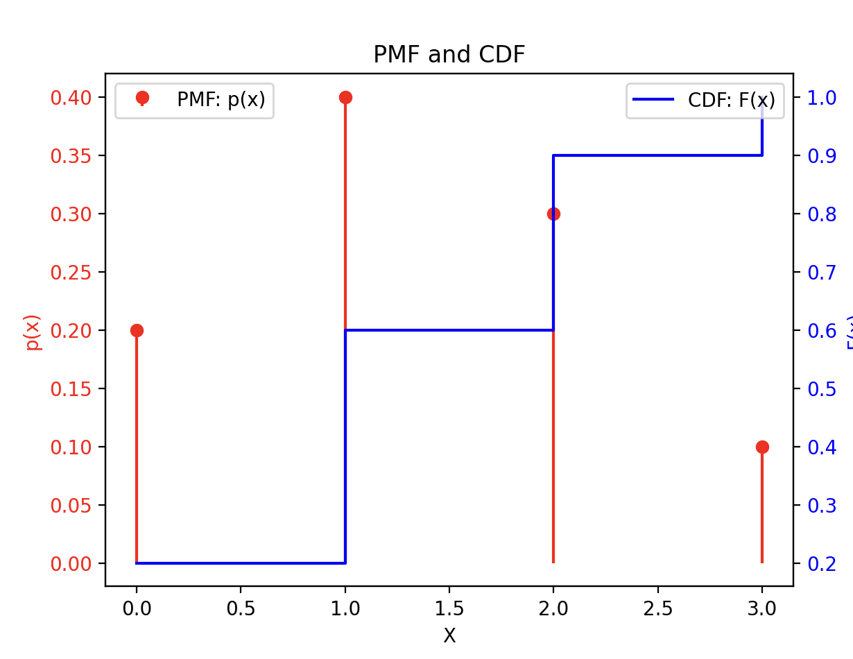
PMF = probability mass function CDF = cumulative distribution function

Let’s make a table.

X	$p(x)=P(X=x)$	$F(x)=P(X\le x)$
0	.2	F(0) = P(X $\le$ 0) = .2
1	.4	F(1) = P(X $\le$ 1) = .6
2	.3	F(2) = P(X $\le$ 2) = .9
3	.1	F(3) = P(X $\le$ 3) = 1
Total	1	F(3) = 1

The probability model for the random variable X is given by the probability mass function (PMF) and the cumulative distribution function (CDF). The PMF gives the probability of each possible value of X, while the CDF gives the probability that X is less than or equal to a given value.

Result: The random variable X represents the number of eggs in the osprey nest, and the probability model for X is given by the PMF and CDF.

python script for plotting PMF and CDF

import micropip
await micropip.install("matplotlib")
import matplotlib.pyplot as plt
 
# Data from the table
X = [0, 1, 2, 3]
p_x = [0.2, 0.4, 0.3, 0.1]  # PMF values
F_x = [0.2, 0.6, 0.9, 1.0]  # CDF values
 
# Create subplots
fig, ax1 = plt.subplots()
 
# Plot PMF (p(x))
ax1.stem(X, p_x, basefmt=" ", linefmt='r-', markerfmt='ro', label='PMF: p(x)', use_line_collection=True)
ax1.set_xlabel('X')
ax1.set_ylabel('p(x)', color='r')
ax1.tick_params(axis='y', labelcolor='r')
 
# Create second y-axis for CDF
ax2 = ax1.twinx()
ax2.step(X, F_x, where='post', label='CDF: F(x)', color='b')
ax2.set_ylabel('F(x)', color='b')
ax2.tick_params(axis='y', labelcolor='b')
 
# Titles and legends
plt.title('PMF and CDF')
ax1.legend(loc='upper left')
ax2.legend(loc='upper right')
 
plt.show()

Definition

Fulcrum: The balancing point of a lever

Question: The Mean of the mass pmf p(x) is the balancing point/fulcrum, called the expected value.

Lets represent this with an equation.

$E(X)=\mu \_x=\sum x\cdot p(x)$

Now let’s make a table of the values.

X	$p(x)=P(X=x)$	$x\cdot p(x)$
0	.2	0
1	.4	.4
2	.3	.6
3	.1	.3
Total	1	1.3

Interesting Fact

The first column of the table is called the support of the random variable X, which is the set of all possible values that X can take.

Result: The expected value of the random variable X is 1.3, which represents the average number of eggs in the osprey nest.

$E(X)=\sum x\cdot p(x)=0\cdot .2+1\cdot .4+2\cdot .3+3\cdot .1=1.3$

---

What this example tells us?

Spread/Variability of the RV’s probability model is the variance.

$Variance=Var(x)=V(X)=\sum (x-\mu {)}^2\cdot p(x)$

This equation gives us the spread or variability of the probability model of the random variable X. The variance measures how much the values of X deviate from the expected value $\mu$.

---

Example 2

Metal cylinder production

A company manufactures metal cylinders that are used in the construction of a particular type of engine. These cylinders, which must slide freely within an outer casing, are designed to have a diameter of 50mm. The company discovers, however, that the cylinders it manufactures can have a diameter anywhere between 49.5 and 50.5. Suppose that the RV, X is the diameter of a randomly chosen cylinder manufactured by the company. Since this random variable can take any value between 49.5 and 50.5, it is a continuous random variable.

Question: What are the diameter’s probability density function and cumulative distribution function?

We are given the following equation:

vertex form of the parabola

• $y=a(x-h{)}^2+k$ → $y=1.5-6(x-50{)}^2$

$f(x)=\{\begin{array}{ll}1.5-6(x-50.0{)}^2,& \text{for }49.5\le x\le 50.5\\ 0,& \text{otherwise}\end{array}$

Graping the PDF with the following python script

import micropip
await micropip.install("numpy")
await micropip.install("matplotlib")
 
import numpy as np
import matplotlib.pyplot as plt
 
# Define the function f(x) for the given parabola
def f(x):
    # Apply the piecewise function
    return np.where((x >= 49.5) & (x <= 50.5), 1.5 - 6 * (x - 50.0)**2, 0)
 
# Generate values for x from 49.4 to 50.6 for plotting (slightly beyond the range to show edges)
x_vals = np.linspace(49.4, 50.6, 400)
y_vals = f(x_vals)
 
# Create the plot
plt.figure(figsize=(6, 4))
plt.plot(x_vals, y_vals, label='PDF of Cylinder Diameter', color='b')
 
# Labeling the plot
plt.title('Probability Density Function of Cylinder Diameter')
plt.xlabel('Diameter (mm)')
plt.ylabel('Probability Density f(x)')
plt.axvline(49.5, color='red', linestyle='--', label='Lower Bound (49.5 mm)')
plt.axvline(50.5, color='green', linestyle='--', label='Upper Bound (50.5 mm)')
 
# Add a legend
plt.legend()
 
# Display the plot
plt.grid(True)
plt.show()

---

Practice for Quiz

To practice for the quiz on this unit, we can practice the Assignment 3 problems 1-6, and apply these methods for the different questions on the quiz.

Visit Quiz Practice - Random Variables for more.

Check out the Axiom page as well